1.2 Multisite stochastic generation of daily precipitation
Wilks (1998) extended the single site stochastic model, described in the previous section, to a multisite model. The basic idea in his
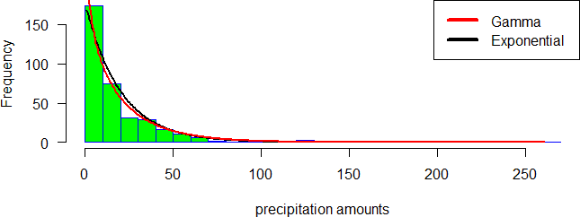
Figure 1.2: Comparison of the histogram for precipitation amounts with the corresponding fitted exponential and gamma probability density functions
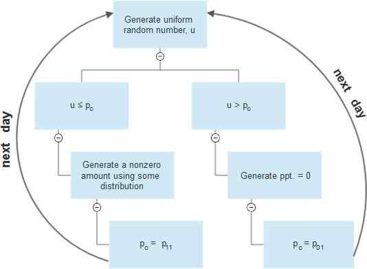
Figure 1.3: Flowcharts for single site daily precipitation generation using two-part model
model is to simultaneously simulate precipitation occurrences using a uniform [0, 1] vector ut and the precipitation amounts using a uniform [0, 1] vector vt in the way in which the elements of ut(k) and vt(k), respectively, are correlated so that
Corr[ut(k), ut(l)] ƒ= 0 and Corr[vt(k), vt(l)] ƒ= 0
for every locations k and l. However, those vectors must be mutually and serially uncorrelated so that
Corr[ut(k), vt(l)] = Corr[ut(k), ut+1(l)] = Corr[vt(k), vt+1(l)] = 0.
1.2.1 Multisite precipitation occurrence process
To simulate precipitation occurrences in a network of K locations, there are K(K−1)/2 pairwise correlations that should be maintained. To achieve the desired correlations, we generate correlated uniform [0, 1] random variates ut whose elements, ut(k), can be derived from standard Gaussian variates wt(k) through the quantile transformation
ut(k) = Φ[wt(k)],
where Φ is the standard normal cumulative distribution function.
Let w(k, l) be the correlation between the station pair k and l so that w(k, l) = Corr[wt(k), wt(l)]. (1.5)
A particular w(k, l) and transition probabilities p01(k) and p11(k) will yield a particular correlation between the synthetic binary series for the two sites,
ξ(k, l) = Corr[Xt(k), Xt(l)]. (1.6)
Denote the observed sample of ξ(k, l) as ξo(k, l) which will have been estimated from the observed binary sequences Xo(k) and Xo(l) t tat locations k and l. Therefore, the desired correlations are achieved by individually finding the K(K − 1)/2 pairwise correlations w(k, l) which, together with the corresponding pairs of transition probabilities, reproduces ξo(k, l) = ξ(k, l) for each pair of stations.
Direct computation of w(k, l) from ξo(k, l) is impossible, because w(k, l) cannot be observed. However, there is a polynomial relationship between w(k, l) and the resulting ξ(k, l) for a given pairs of transition probabilities. Figure 1.4 shows an example of such a relationship, computed using stochastic simulation.
This relationship can be estimated using polynomial regression. Figure 1.5 illustrates the estimated polynomial function.
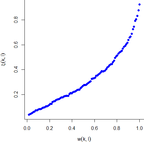
Figure 1.4: An example of the relationship between w(k, l) and ξ(k, l)
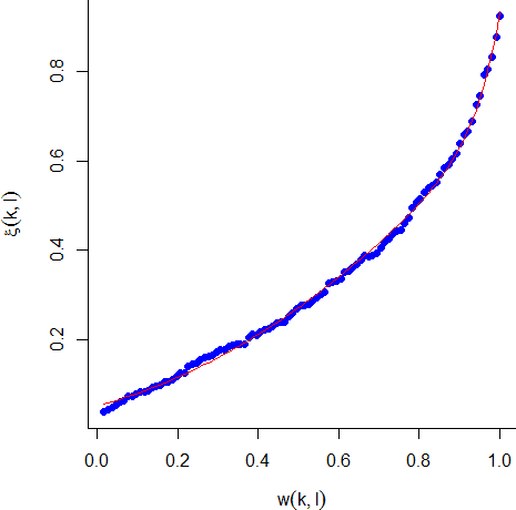
Figure 1.5: Estimation of the relationship between w(k, l) and ξ(k, l) using polynomial regression
Let f be the estimated function of the relationship between w(k, l) and ξ(k, l) so that
f [w(k, l)] = ξ(k, l).
To solve the first aspect of the precipitation generation problem, we use a nonlinear root finding algorithm by defining the function
Q[w(k, l)] = f [w(k, l)] − ξo(k, l) and finding the w(k, l) for which Q[w(k, l)] = 0.
The wt(k) are generated using a multivariate normal distribution vector wt having mean vector 0 and variance-covariance matrix [Σ] the elements of which are the correlations w(k, l)(see Appendix B).
The resulting individual wt(k) will be distributed as univariate standard normal distribution and may be used to generate precipitation occurrence time series Xt(k) using. 1 if wt(k) ≤ Φ−1[pc(k)]
This process of simultaneously simulate occurrences using multivariate normal distribution defined by the K(K − 1)/2 pairwise correlations, was referred to as the hidden covariance model (Srikanthan and Pegram, 2006).
1.2.2 Multisite precipitation amounts process
The precipitation amounts on wet days are generated using the Gamma distribution, which has been found to fit the observed sequences better than the exponential distribution.
As was the case for the occurrence model, it is crucial to consider the spatial carrelations between all locations in the simulation process.
After estimating the parameters of the Gamma distribution at each location, we generate a vector of random uniform variates vt whose elements vt(k) are cross correlated but serially independent and can be derived from standard Gaussian variates zt(k) through the quantile transformation vt(k) = Φ[zt(k)].
Then the precipitation amounts are generated by inversion using where G is the inverse of the cumulated distribution function of the Gamma distribution.
rt(k) = rmin + G(vt(k)), (1.8)
The vector zt is drawn from a multivariate normal distribution with mean vector 0 and variance-covariance matrix [Ω], whose elements are:
ζ(k, l) = Corr[zt(k), zt(l)], (1.9)
Direct computation of [Ω] from the observed precipitation data is not possible. Let η(k, l) be the cross correlations between daily precipitation at locations k and l such that
η(k, l) = Corr[Yt(k), Yt(l)] (1.10)
Denote the observed sample of η(k, l) as ηo(k, l) which will have been estimated from the observed sequences Y o(k) and Y o(l) at locations k and l. As in the case of simulating precipitation occurrences, in a network of K locations, there are K(K − 1)/2 pairwise correlations that should be preserved in the simulation process.
t t
The relationship between η(k, l) and ζ(k, l) is linear. Figure 1.6 illustrates this relationship, obtained using stochastic simulation, and its estimation using linear regression.
After choosing the appropriate correlation structure of the multivariate normal distribution, defined by the equations in 1.9, nonzero amounts are generated using equation 1.8.
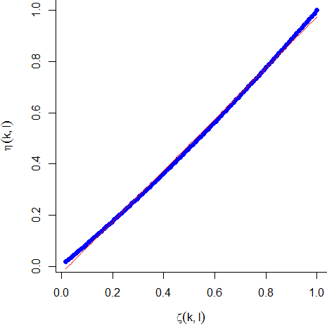
Figure 1.6: The relationship between η(k, l) and ζ(k, l)