3 Application
3.1 Data
The data used in this study, is the daily rainfalls at 6 stations in Scotland (table 3.1), from 1 January 1961 to 31 December 2015.
This data is used to simultaneously simulate daily, monthly and annual precipitation at the 6 locations.
The data is available in the National River Flow Archive website https://nrfa.ceh.ac.uk/data/search.
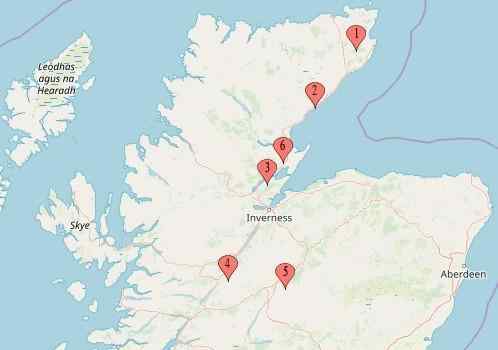
Figure 3.1: Stations numbers and their locations on map.
| Station Number | Location | Catchement Area (km2) |
| 1 | Tarroul | 161.9 |
| 2 | Kilphedir | 551.4 |
| 3 | Alness | 201 |
| 4 | Ardachy Bridge | 75.9 |
| 5 | Glenmeanie | 120.5 |
| 6 | Fasnakyle | 277.5 |
Table 3.1: Location and catchement area of stations
3.2 Daily simulations
The method described in section 1.2 is used to simultaneously simulate daily sequences of precipitation at the 6 locations. To preserve the seasonal characteristics of the observed time series, each calendar month is considered separately in the model.
At first the daily occurrences are generated using the multisite occurrence process at all stations, then the daily amounts are generated using the Gamma distribution.
3.2.1 Daily occurrence process
In this section, the occurrence process model is used to generate the daily occurrences at all locations.
In figure 3.2, the spatial correlations of the observed daily occurrences are compared with the generated ones. The spatial correlations are well represented by the model with some errors resulted during the simulation process.
3.2.2 Daily amounts process
As described in section 1.2, nonzero precipitation amounts are modeled using the Gamma distribution, whose parameters are estimated, for each site at each calendar month, using the maximum likelihood estimation.
The Gamma distribution is fitted to nonzero amounts of station 1 in January, and the P-value resulted from the Kolmogorov Smirnov test is 0.7.
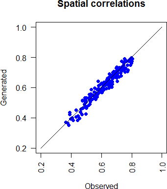
Figure 3.2: Comparison of generated and observed spatial correlations of daily rainfall occurrences.
The empirical and theoretical densities, CDFs, quantiles, and probabilities for the same time series are compared in figure 3.3, 3.4, and 3.5. Thus, the Gamma distribution fit well the nonzero amounts.
The generated spatial correlations are compared with the observed ones in figure 3.6, and they are well represented by the model.
It is of interest to examine the degree to which the daily precipitation occurrence and amounts models reproduce the statistics of observed precipitation climate on longer time scales. Therefore, various monthly statistics are investigated.
Figure 3.7 shows the relationship between generated and observed mean precipitation, for all 6 stations and all 12 months.
Similarly, figure 3.8, and 3.8 show respectively, the standard deviations of monthly precipitation (characterizing the interannual variation in total monthly precipitation) in the observations versus generated series and the observed median of monthly precipitation versus the simulated ones.
The statistics of daily rainfalls on long time scales are therefore well reproduced by the two part model.
Figure 3.10 shows the box plot for observed and generated daily precipitation at station 5 and 6 at all 12 months. The skewness and quartiles are well represented by the two part model. The variability is also well reproduced by the model, which confirms the results in figure 3.8.
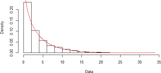
Figure 3.3: Comparison of empirical and theoretical densities.
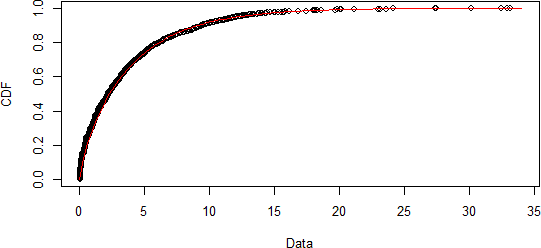
Figure 3.4: Comparison of empirical and theoretical CDFs.
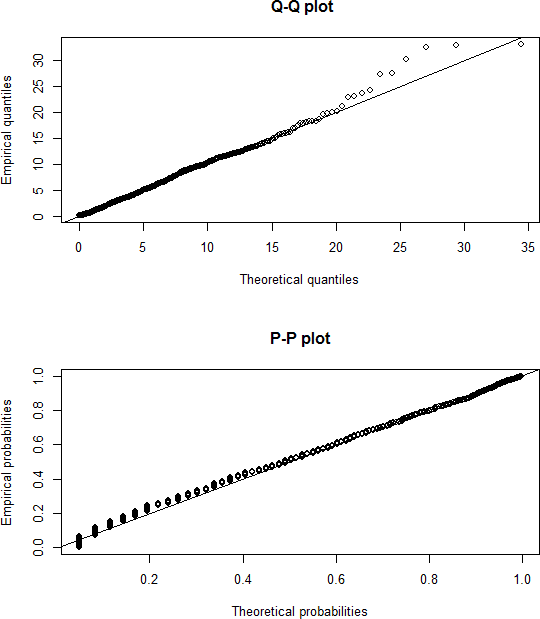
Figure 3.5: Q-Q plot and P-P plot.
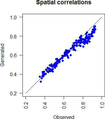
Figure 3.6: Comparison of generated and observed spatial correlations of daily rainfall amounts.
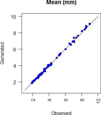
Figure 3.7: Comparison of generated and observed mean monthly rainfall at all stations and all months.
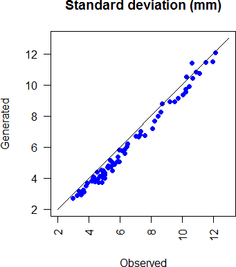
Figure 3.8: Comparison of generated and observed monthly s.d. rainfall at all stations and all months.
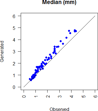
Figure 3.9: Comparison of generated and observed monthly median rainfall at all stations and all months.
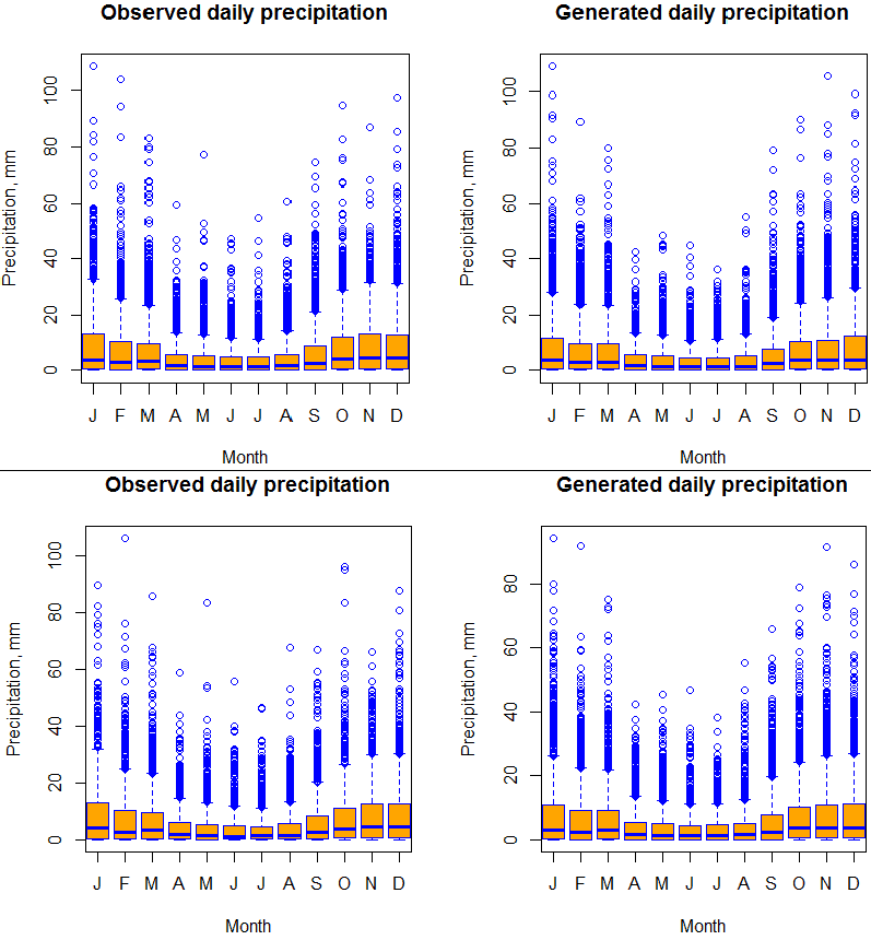
Figure 3.10: Box plot of the observed and generated daily precipitation at all 12 months, at station 6 for the top panel and station 5 for the bottom panel.
3.3 Monthly simulations
As described in section 2.2, to generate monthly precipitation, daily rainfall amounts are aggregated into monthly totals and they are modified using a lag one vector autoregressive process.
The nested model is used to preserve the monthly characteristics; therefore, it is crucial to examine how well this model represents the monthly statistics.
Figure 3.11 shows the times series of observed and adjusted generated monthly precipitation at station 3 on month August.
The spatial correlations of the generated monthly totals and the adjusted generated monthly totals are compared with the observed ones in figure 3.12. The multisite nested model performs better in representing the spatial correlations.
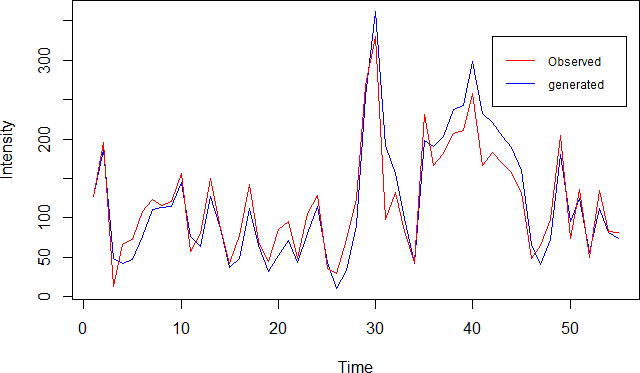
Figure 3.11: Comparison of generated and observed monthly precipitation time series at station 3 on month August.
Figure 3.13, 3.14, and 3.15 show, respectively, the observed monthly precipitation means versus the generated ones (using the nested model), the observed monthly precipitation standard deviations versus the generated ones, and the observed monthly precipitation medians versus the generated ones.
Those statistics are well
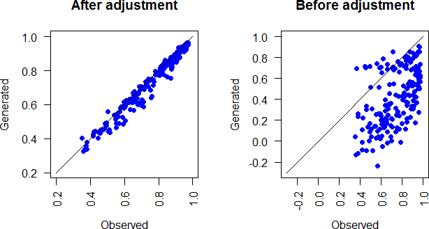
Figure 3.12: Comparison of generated and observed monthly spatial correlations for all months. right panel: spatial correlations before adjustment, left panel: spatial correlations after adjustment.
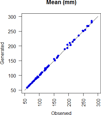
Figure 3.13: Comparison of generated and observed monthly rainfall means for all months at all stations.
represented by the model.
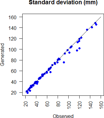
Figure 3.14: Comparison of generated and observed monthly rainfall s.d, for all months at all stations.
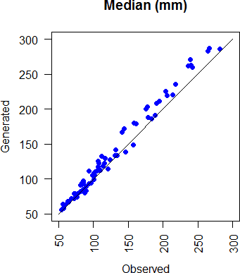
Figure 3.15: Comparison of generated and observed monthly rainfall medians for all months at all stations.
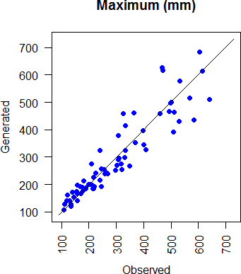
Figure 3.16: Comparison of generated and observed monthly rainfall maximum for all months at all stations.
The maximum monthly rainfalls at stations with a monthly maximum values less than 300 are well represented by the model. Whereas, for the stations with maximum values greater than 300, the model tends to underestimate and overestimate the statistic (figure 3.16).
3.4 Annual simulations
After generating the monthly precipitation using the nested model, the annual totals are obtained by aggregating the monthly simulations. Then those annual totals are modified by a lag one vector autoregressive model.
Figure 3.17 shows the times series of observed and adjusted generated annual precipitation at station 6 for all the 55 years.
The spatial correlations of the annual rainfall totals and the adjusted annual rainfall totals are compared with the observed ones in figure 3.18. This figure shows a better performance of the nested model in representing the spatial correlations.
Various other statistics are investigated here, such as the mean, standard deviation, median, maximum, and minimum of annual precipitation at all locations (figure 3.19, 3.20, 3.21, 3.22, and 3.23 respectively). All the statistics are well represented by the multisite annual model.
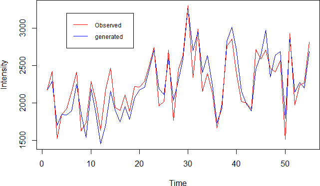
Figure 3.17: Comparison of generated and observed annual rainfall time series at station 6.
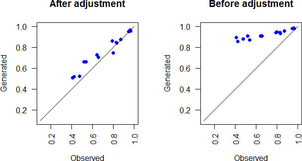
Figure 3.18: Comparison of generated and observed annual rainfall spatial correlations. right panel: spatial correlations before adjustment, left panel: spatial correlations after adjustment.
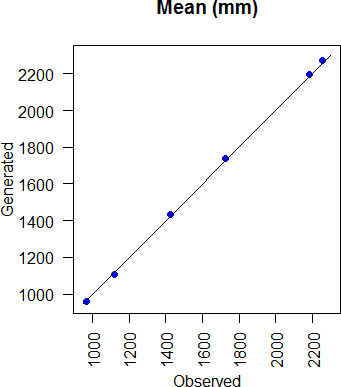
Figure 3.19: Comparison of generated and observed annual rainfall means for all stations.
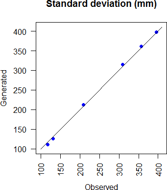
Figure 3.20: Comparison of generated and observed annual rainfall s.d. for all stations.
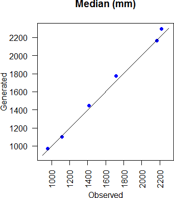
Figure 3.21: Comparison of generated and observed annual rainfall median for all stations.
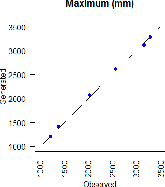
Figure 3.22: Comparison of generated and observed annual rainfall maximum for all stations.
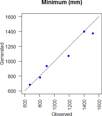
Figure 3.23: Comparison of generated and observed annual rainfall minimum for all stations.
The multisite two part model, developed by Wilks (1998), was used to simultaneously generate daily precipitation at 6 locations in Scotland. As its name indicates, the two part model is consisting of two parts, namely, the occurrence process and the amounts process.
The occurrence process was modeled using a first-order twostage Markov chain and the amounts process was modeled using the Gamma distribution. In the multisite contexte, it is important to consider the spatial correlations between the locations.
To preserve the spatial correlations, daily occurrences were simulated using Uniform variates derived from a multivariate normal distribution and use a root finding algorithm (bisection) to find the correlation structure of the MVN that gives the desired correlations. The same method was used to generate the nonzero amounts.
The model was effective in preserving the spatial correlations and other statistics such as the mean, the standard deviation, and the median. Although this model does well in representing the daily statistics, it fails in representing the monthly and annual ones (figure 3.12 and 3.18).
To address this issue, the nested model (Srikanthan, 2009) was used to adjust the generated monthly and annual rainfall totals at the 6 locations. At first, to simulate monthly rainfalls, the generated daily precipitation sequences were aggregated into monthly toatals, and they were nested using a lag one vector autoregressive model. Then those monthly simulations were aggregated into annual totals, and they were in turn modified using a lag one vector autoregressive model.
For monthly simulations, the nested model was effective in reproducing the monthly statistics in all locations, except the maximum. The annual statistics were also well represented by the nested model, including the maximum and minimum annual rainfalls. A Maximum likelihood estimation of transition probabilities
Consider a Markov chain (X1∞
= Xt, t = 0, 1, …) with m states, we want to estimate the transition matrix from the observed data
n ≡ x1, x2, …, xn. The elements of the transition matrix pij are defined as
pij = Pr(Xt+1 = j|Xt = i).
The probability of the realization of X1∞ is
1 1 1 1
t=2 n
= Pr(X1 = x1) Pr(Xt = xt|Xt−1 = xt−1) (A.2)
t=2 n
= Pr(X1 = x1) pxt−1xt (A.3)
t=2
Equation A.1 uses the definition of conditional probabilities and Equation A.2 uses the Markov propriety.
Denote p the transition probabilities such that
p = (pij, i = 1, …, m, j = 1, …, m)
Define the transition counts nij number of times i is followed by j in Xn. Thus, the likelihood function of a given transition probabilities is defined as
m m
L(p) = Pr(X1 = x1) Y Y pnij
(A.4)
and the log-likelihood function as
i=1 j=1
L(p) = log[L(p)] = log[Pr(X1 = x1)] + nij log(pij) (A.5)
i,j
We want to maximize L under the m constraint equations
pij = 1, i = 1, …, m. (A.6)
j
Using m Lagrange multipliers, λ = (λ1, λ2, …, λm), the new objective function is
f (p, λ) = L(p) − Σ λi( Σ pij − 1 ) (A.7)
The resulting estimations of transition probabilities, after maximizing the objective function f, are
pˆij =
nij
m j=1
nij
(A.8)
B Simulation of multivariate normal distribution
Let z1, …, zm be independent and identically distributed normal variates with mean 0 and variance 1. If for constants aij, i = 1, …, n j = 1, …, m
w1 = a11z1 + a12z2 + … + a1mzm w2 = a21z1 + a22z2 + … + a2mzm
wn = an1z1 + an2z2 + … + anmzm
which is equivalent to w = AzJ, where A = (aij) i=1,…,n j=1,…,m, then the vector w = (w1, w2, …, wn) is said to have a multivariate normal distribution such that
m
E(wi) = 0 and Cov(wi, wj) = aikajk∀ 1 ≤ i, j ≤ n (B.1)
k=1
Equation B.1 is equivalent to Σ = AtA, where Σ is the variancecovariance matrix.
Therefore, to generate the multivariate normal distribution, we first find a matrix A such that Σ = AtA using Choleski decomposition or singular value decomposition and then generate independent standard normal variates z1, z2, …, zn and set w = AzJ.
C Implementation of the models in R
All the models used in this study were implemented in R. The functions I used are available in my Github account: https://github.com/SaidObakrim/Multisite-generation-of-daily-precipitation
[1] Ailliot, P., Allard, D., Monbet, V., and Naveau, P (2015) Stochastic weather generators: an overview of weather type models, J. Soc. Franc. Stat., 156, 101–113, 2015.
[2] Matalas, N.C. (1967) Mathematical assessment of synthetic hydrology. Water Resources Research 3 (4), 937–945.
[3] Martin Haugh (2007) Generating Random Variables and Stochastic Processes
[4] Srikanthan, R. (2005) Stochastic generation of daily rainfall and at a number of sites, Technical Report 05/7, CRC for Catchment Hydrology, Monash University, Victoria
[5] Srikanthan, R. (2006) Stochastic generation of spatially consistent daily rainfall at multiple sites. 30th Hydrology and Water Resources Symposium, Launceston.
[6] Srikanthan, R. and G. G. S. Pegram (2006) Stochastic generation of multisite rainfall occurrence. Advances in Geosciences, Vol. 6, 1-10.
[7] Srikanthan, R. and G. G. S. Pegram StochasticGeneration of Spatially Consistent Dail Rainfall.
[8] Srikanthan, R. and G. G. S. Pegram (2009) A nested multisite daily rainfall stochastic generation model. Journal of Hydrology 371 142–153
[9] Wilks, D. S. (1998) Multisite generalisation of a daily stochastic precipitation generation model. Journal of Hydrology 210: 178-191.
[10] Wilks, D. S. and Wilby, R. L. (1999) The weather generation game: a review of stochastic weather models, Prog. Phys. Geogr., 23, 329–357.